

在Iris数据集上绘制树集成的决策曲面
使用Iris数据集的一对特征训练随机树的森林, 并绘制决策界面。
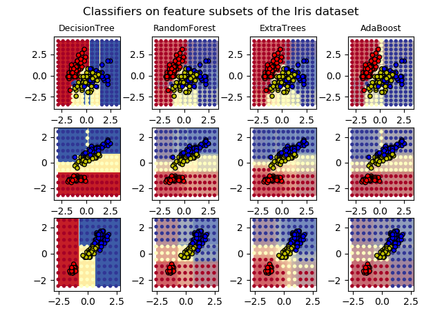
此图比较了决策树分类器(第一列)、随机森林分类器(第二列)、极端树分类器(第三列)和AdaBoost分类器(第四列)学习的决策面。
在第一行中,分类器只使用萼片宽度和萼片长度特征,第二行仅使用花瓣长度和萼片长度,第三行仅使用花瓣宽度和花瓣长度。
按照得分的降序,当使用30个估计器对所有4个特性进行训练(在本示例之外)并使用10倍交叉验证得分时,我们看到:
ExtraTreesClassifier()  # 0.95 score
RandomForestClassifier()  # 0.94 score
AdaBoost(DecisionTree(max_depth=3))  # 0.94 score
DecisionTree(max_depth=None)  # 0.94 score
增加AdaBoost的 max_depth会降低分数的标准差(但平均分数没有提高)。
有关每个模型的更多细节,请参见控制台的输出。
在本例中,您可以尝试:
对于 DecisionTreeClassifier和AdaBoostClassifier, 可以改变max_depth, 或许可以尝试对于DecisionTreeClassifiermax_depth=3, 而对于AdaBoostClassifier可以是max_depth=None。改变 n_estimators。
值得注意的是,RandomForests和ExtraTrees可以在许多内核上并行训练,因为每棵树都是独立于其他树构建的。AdaBoost的树是按顺序构建的,因此不要使用多个核。
DecisionTree with features [0, 1] has a score of 0.9266666666666666
RandomForest with 30 estimators with features [0, 1] has a score of 0.9266666666666666
ExtraTrees with 30 estimators with features [0, 1] has a score of 0.9266666666666666
AdaBoost with 30 estimators with features [0, 1] has a score of 0.8533333333333334
DecisionTree with features [0, 2] has a score of 0.9933333333333333
RandomForest with 30 estimators with features [0, 2] has a score of 0.9933333333333333
ExtraTrees with 30 estimators with features [0, 2] has a score of 0.9933333333333333
AdaBoost with 30 estimators with features [0, 2] has a score of 0.9933333333333333
DecisionTree with features [2, 3] has a score of 0.9933333333333333
RandomForest with 30 estimators with features [2, 3] has a score of 0.9933333333333333
ExtraTrees with 30 estimators with features [2, 3] has a score of 0.9933333333333333
AdaBoost with 30 estimators with features [2, 3] has a score of 0.9933333333333333
print(__doc__)

import numpy as np
import matplotlib.pyplot as plt
from matplotlib.colors import ListedColormap

from sklearn.datasets import load_iris
from sklearn.ensemble import (RandomForestClassifier, ExtraTreesClassifier,
                              AdaBoostClassifier)
from sklearn.tree import DecisionTreeClassifier

# Parameters
n_classes = 3
n_estimators = 30
cmap = plt.cm.RdYlBu
plot_step = 0.02  # fine step width for decision surface contours
plot_step_coarser = 0.5  # step widths for coarse classifier guesses
RANDOM_SEED = 13  # fix the seed on each iteration

# Load data
iris = load_iris()

plot_idx = 1

models = [DecisionTreeClassifier(max_depth=None),
          RandomForestClassifier(n_estimators=n_estimators),
          ExtraTreesClassifier(n_estimators=n_estimators),
          AdaBoostClassifier(DecisionTreeClassifier(max_depth=3),
                             n_estimators=n_estimators)]

for pair in ([0, 1], [0, 2], [2, 3]):
    for model in models:
        # We only take the two corresponding features
        X = iris.data[:, pair]
        y = iris.target

        # Shuffle
        idx = np.arange(X.shape[0])
        np.random.seed(RANDOM_SEED)
        np.random.shuffle(idx)
        X = X[idx]
        y = y[idx]

        # Standardize
        mean = X.mean(axis=0)
        std = X.std(axis=0)
        X = (X - mean) / std

        # Train
        model.fit(X, y)

        scores = model.score(X, y)
        # Create a title for each column and the console by using str() and
        # slicing away useless parts of the string
        model_title = str(type(model)).split(
            ".")[-1][:-2][:-len("Classifier")]

        model_details = model_title
        if hasattr(model, "estimators_"):
            model_details += " with {} estimators".format(
                len(model.estimators_))
        print(model_details + " with features", pair,
              "has a score of", scores)

        plt.subplot(3, 4, plot_idx)
        if plot_idx <= len(models):
            # Add a title at the top of each column
            plt.title(model_title, fontsize=9)

        # Now plot the decision boundary using a fine mesh as input to a
        # filled contour plot
        x_min, x_max = X[:, 0].min() - 1, X[:, 0].max() + 1
        y_min, y_max = X[:, 1].min() - 1, X[:, 1].max() + 1
        xx, yy = np.meshgrid(np.arange(x_min, x_max, plot_step),
                             np.arange(y_min, y_max, plot_step))

        # Plot either a single DecisionTreeClassifier or alpha blend the
        # decision surfaces of the ensemble of classifiers
        if isinstance(model, DecisionTreeClassifier):
            Z = model.predict(np.c_[xx.ravel(), yy.ravel()])
            Z = Z.reshape(xx.shape)
            cs = plt.contourf(xx, yy, Z, cmap=cmap)
        else:
            # Choose alpha blend level with respect to the number
            # of estimators
            # that are in use (noting that AdaBoost can use fewer estimators
            # than its maximum if it achieves a good enough fit early on)
            estimator_alpha = 1.0 / len(model.estimators_)
            for tree in model.estimators_:
                Z = tree.predict(np.c_[xx.ravel(), yy.ravel()])
                Z = Z.reshape(xx.shape)
                cs = plt.contourf(xx, yy, Z, alpha=estimator_alpha, cmap=cmap)

        # Build a coarser grid to plot a set of ensemble classifications
        # to show how these are different to what we see in the decision
        # surfaces. These points are regularly space and do not have a
        # black outline
        xx_coarser, yy_coarser = np.meshgrid(
            np.arange(x_min, x_max, plot_step_coarser),
            np.arange(y_min, y_max, plot_step_coarser))
        Z_points_coarser = model.predict(np.c_[xx_coarser.ravel(),
                                         yy_coarser.ravel()]
                                         ).reshape(xx_coarser.shape)
        cs_points = plt.scatter(xx_coarser, yy_coarser, s=15,
                                c=Z_points_coarser, cmap=cmap,
                                edgecolors="none")

        # Plot the training points, these are clustered together and have a
        # black outline
        plt.scatter(X[:, 0], X[:, 1], c=y,
                    cmap=ListedColormap(['r', 'y', 'b']),
                    edgecolor='k', s=20)
        plot_idx += 1  # move on to the next plot in sequence

plt.suptitle("Classifiers on feature subsets of the Iris dataset", fontsize=12)
plt.axis("tight")
plt.tight_layout(h_pad=0.2, w_pad=0.2, pad=2.5)
plt.show()
脚本的总运行时间:(0分9.465秒)

