

GMM协方差
高斯混合模型几种协方差类型的证明。
有关估计器的更多信息,请参见高斯混合模型。
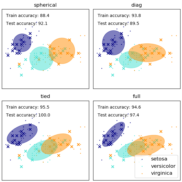
虽然GMM经常用于聚类,但我们可以将所获得的聚类与数据集中的实际类进行比较。我们用训练集中的类均值初始化高斯的均值,以使这种比较有效。
我们在iris数据集上使用多种GMM协方差类型, 并绘制了在训练集和测试集上的预测标签。我们比较了球形的、对角的、完全的、关联的协方差矩阵的GMM性能增加的顺序进行比较。虽然通常预计完全协方差表现最好,但在小数据集上往往会出现过拟合,并且不能很好地泛化到测试数据。在图中,训练数据显示为圆点,而测试数据显示为叉。iris数据集是四维的。这里只显示了前两个维度,因此一些点在其他维度中被分开。
# Author: Ron Weiss <ronweiss@gmail.com>, Gael Varoquaux
# Modified by Thierry Guillemot <thierry.guillemot.work@gmail.com>
# License: BSD 3 clause

import matplotlib as mpl
import matplotlib.pyplot as plt

import numpy as np

from sklearn import datasets
from sklearn.mixture import GaussianMixture
from sklearn.model_selection import StratifiedKFold

print(__doc__)

colors = ['navy', 'turquoise', 'darkorange']


def make_ellipses(gmm, ax):
    for n, color in enumerate(colors):
        if gmm.covariance_type == 'full':
            covariances = gmm.covariances_[n][:2, :2]
        elif gmm.covariance_type == 'tied':
            covariances = gmm.covariances_[:2, :2]
        elif gmm.covariance_type == 'diag':
            covariances = np.diag(gmm.covariances_[n][:2])
        elif gmm.covariance_type == 'spherical':
            covariances = np.eye(gmm.means_.shape[1]) * gmm.covariances_[n]
        v, w = np.linalg.eigh(covariances)
        u = w[0] / np.linalg.norm(w[0])
        angle = np.arctan2(u[1], u[0])
        angle = 180 * angle / np.pi  # convert to degrees
        v = 2. * np.sqrt(2.) * np.sqrt(v)
        ell = mpl.patches.Ellipse(gmm.means_[n, :2], v[0], v[1],
                                  180 + angle, color=color)
        ell.set_clip_box(ax.bbox)
        ell.set_alpha(0.5)
        ax.add_artist(ell)
        ax.set_aspect('equal', 'datalim')

iris = datasets.load_iris()

# Break up the dataset into non-overlapping training (75%) and testing
# (25%) sets.
skf = StratifiedKFold(n_splits=4)
# Only take the first fold.
train_index, test_index = next(iter(skf.split(iris.data, iris.target)))


X_train = iris.data[train_index]
y_train = iris.target[train_index]
X_test = iris.data[test_index]
y_test = iris.target[test_index]

n_classes = len(np.unique(y_train))

# Try GMMs using different types of covariances.
estimators = {cov_type: GaussianMixture(n_components=n_classes,
              covariance_type=cov_type, max_iter=20, random_state=0)
              for cov_type in ['spherical', 'diag', 'tied', 'full']}

n_estimators = len(estimators)

plt.figure(figsize=(3 * n_estimators // 2, 6))
plt.subplots_adjust(bottom=.01, top=0.95, hspace=.15, wspace=.05,
                    left=.01, right=.99)


for index, (name, estimator) in enumerate(estimators.items()):
    # Since we have class labels for the training data, we can
    # initialize the GMM parameters in a supervised manner.
    estimator.means_init = np.array([X_train[y_train == i].mean(axis=0)
                                    for i in range(n_classes)])

    # Train the other parameters using the EM algorithm.
    estimator.fit(X_train)

    h = plt.subplot(2, n_estimators // 2, index + 1)
    make_ellipses(estimator, h)

    for n, color in enumerate(colors):
        data = iris.data[iris.target == n]
        plt.scatter(data[:, 0], data[:, 1], s=0.8, color=color,
                    label=iris.target_names[n])
    # Plot the test data with crosses
    for n, color in enumerate(colors):
        data = X_test[y_test == n]
        plt.scatter(data[:, 0], data[:, 1], marker='x', color=color)

    y_train_pred = estimator.predict(X_train)
    train_accuracy = np.mean(y_train_pred.ravel() == y_train.ravel()) * 100
    plt.text(0.05, 0.9, 'Train accuracy: %.1f' % train_accuracy,
             transform=h.transAxes)

    y_test_pred = estimator.predict(X_test)
    test_accuracy = np.mean(y_test_pred.ravel() == y_test.ravel()) * 100
    plt.text(0.05, 0.8, 'Test accuracy: %.1f' % test_accuracy,
             transform=h.transAxes)

    plt.xticks(())
    plt.yticks(())
    plt.title(name)

plt.legend(scatterpoints=1, loc='lower right', prop=dict(size=12))


plt.show()
脚本的总运行时间:(0分0.223秒)

