

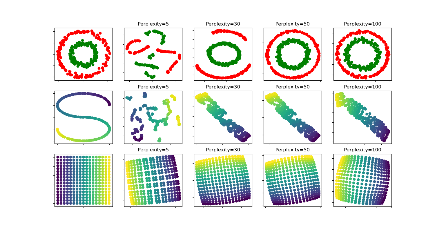
t-sne:不同perplexity值对形状的影响
两个同心圆和S曲线数据集对不同perplexity值的t-SNE的说明。
我们观察到,随着perplexity值的增加,形状越来越清晰。
聚类的大小、距离和形状可能因初始化、perplexity值而异,并不总是能够传达意义。
如下所示,对于较高的perplexity,t-SNE发现了两个同心圆的有意义的拓扑结构,但圆圈的大小和距离与原来的略有不同。与这两个圆数据集相反,即使在较大的perplexity值下,形状在视觉上也与S曲线数据集上的S曲线拓扑不同。
更多细节, “如何有效地使用t-SNE” https://distill.pub/2016/misread-tsne/提供了一个很好的关于各种参数的影响的讨论,以及互动的情节。
circles, perplexity=5 in 1.6 sec
circles, perplexity=30 in 2.2 sec
circles, perplexity=50 in 2.3 sec
circles, perplexity=100 in 2.5 sec
S-curve, perplexity=5 in 1.7 sec
S-curve, perplexity=30 in 2.3 sec
S-curve, perplexity=50 in 1.9 sec
S-curve, perplexity=100 in 2.7 sec
uniform grid, perplexity=5 in 1.5 sec
uniform grid, perplexity=30 in 2.1 sec
uniform grid, perplexity=50 in 1.9 sec
uniform grid, perplexity=100 in 2.7 sec
# Author: Narine Kokhlikyan <narine@slice.com>
# License: BSD

print(__doc__)

import numpy as np
import matplotlib.pyplot as plt

from matplotlib.ticker import NullFormatter
from sklearn import manifold, datasets
from time import time

n_samples = 300
n_components = 2
(fig, subplots) = plt.subplots(3, 5, figsize=(15, 8))
perplexities = [5, 30, 50, 100]

X, y = datasets.make_circles(n_samples=n_samples, factor=.5, noise=.05)

red = y == 0
green = y == 1

ax = subplots[0][0]
ax.scatter(X[red, 0], X[red, 1], c="r")
ax.scatter(X[green, 0], X[green, 1], c="g")
ax.xaxis.set_major_formatter(NullFormatter())
ax.yaxis.set_major_formatter(NullFormatter())
plt.axis('tight')

for i, perplexity in enumerate(perplexities):
    ax = subplots[0][i + 1]

    t0 = time()
    tsne = manifold.TSNE(n_components=n_components, init='random',
                         random_state=0, perplexity=perplexity)
    Y = tsne.fit_transform(X)
    t1 = time()
    print("circles, perplexity=%d in %.2g sec" % (perplexity, t1 - t0))
    ax.set_title("Perplexity=%d" % perplexity)
    ax.scatter(Y[red, 0], Y[red, 1], c="r")
    ax.scatter(Y[green, 0], Y[green, 1], c="g")
    ax.xaxis.set_major_formatter(NullFormatter())
    ax.yaxis.set_major_formatter(NullFormatter())
    ax.axis('tight')

# Another example using s-curve
X, color = datasets.make_s_curve(n_samples, random_state=0)

ax = subplots[1][0]
ax.scatter(X[:, 0], X[:, 2], c=color)
ax.xaxis.set_major_formatter(NullFormatter())
ax.yaxis.set_major_formatter(NullFormatter())

for i, perplexity in enumerate(perplexities):
    ax = subplots[1][i + 1]

    t0 = time()
    tsne = manifold.TSNE(n_components=n_components, init='random',
                         random_state=0, perplexity=perplexity)
    Y = tsne.fit_transform(X)
    t1 = time()
    print("S-curve, perplexity=%d in %.2g sec" % (perplexity, t1 - t0))

    ax.set_title("Perplexity=%d" % perplexity)
    ax.scatter(Y[:, 0], Y[:, 1], c=color)
    ax.xaxis.set_major_formatter(NullFormatter())
    ax.yaxis.set_major_formatter(NullFormatter())
    ax.axis('tight')


# Another example using a 2D uniform grid
x = np.linspace(0, 1, int(np.sqrt(n_samples)))
xx, yy = np.meshgrid(x, x)
X = np.hstack([
    xx.ravel().reshape(-1, 1),
    yy.ravel().reshape(-1, 1),
])
color = xx.ravel()
ax = subplots[2][0]
ax.scatter(X[:, 0], X[:, 1], c=color)
ax.xaxis.set_major_formatter(NullFormatter())
ax.yaxis.set_major_formatter(NullFormatter())

for i, perplexity in enumerate(perplexities):
    ax = subplots[2][i + 1]

    t0 = time()
    tsne = manifold.TSNE(n_components=n_components, init='random',
                         random_state=0, perplexity=perplexity)
    Y = tsne.fit_transform(X)
    t1 = time()
    print("uniform grid, perplexity=%d in %.2g sec" % (perplexity, t1 - t0))

    ax.set_title("Perplexity=%d" % perplexity)
    ax.scatter(Y[:, 0], Y[:, 1], c=color)
    ax.xaxis.set_major_formatter(NullFormatter())
    ax.yaxis.set_major_formatter(NullFormatter())
    ax.axis('tight')


plt.show()
脚本的总运行时间:(0分26.425秒)

