

核岭回归与SVR的比较
内核岭回归(KRR)和SVR都通过采用内核技巧来学习非线性函数,即,它们在由相应内核诱导的空间中学习了与原始空间中的非线性函数相对应的线性函数。它们在损失函数上有所不同(脊波与对ε无关的损失)。与SVR相比,KRR的拟合可以封闭形式进行,对于中等规模的数据集通常更快。另一方面,学习的模型是非稀疏的,因此在预测时比SVR慢。
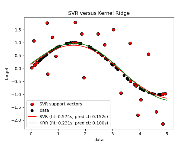
此示例说明了人工数据集上的两种方法,该方法由正弦目标函数和添加到每五个数据点的强噪声组成。第一张图比较了当使用网格搜索优化RBF内核的复杂度/正则化和带宽时,KRR和SVR的学习模型。学习的功能非常相似。但是,拟合KRR约为。比安装SVR快7倍(两者都使用网格搜索)。但是,使用SVR预测100000个目标值的速度快了树倍以上,因为它仅使用了大约10个像素就学会了稀疏模型。 100个训练数据点的1/3作为支持向量。
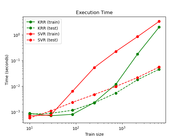
下图比较了不同大小的训练集的KRR和SVR的拟合和预测时间。对于中型训练集(少于1000个样本),拟合KRR比SVR快。但是,对于较大的训练集,SVR的缩放范围更好。关于预测时间,由于学习到的稀疏解决方案,对于所有规模的训练集,SVR均比KRR更快。注意,稀疏度以及预测时间取决于SVR的参数ε和C。
# 作者: Jan Hendrik Metzen <jhm@informatik.uni-bremen.de>
# 执照: BSD 3 clause


import time

import numpy as np

from sklearn.svm import SVR
from sklearn.model_selection import GridSearchCV
from sklearn.model_selection import learning_curve
from sklearn.kernel_ridge import KernelRidge
import matplotlib.pyplot as plt

rng = np.random.RandomState(0)

# #############################################################################
# 获得样本数据
X = 5 * rng.rand(10000, 1)
y = np.sin(X).ravel()

# 对目标增加噪音
y[::5] += 3 * (0.5 - rng.rand(X.shape[0] // 5))

X_plot = np.linspace(0, 5, 100000)[:, None]

# #############################################################################
# 拟合回归模型
train_size = 100
svr = GridSearchCV(SVR(kernel='rbf', gamma=0.1),
                   param_grid={"C": [1e0, 1e1, 1e2, 1e3],
                               "gamma": np.logspace(-2, 2, 5)})

kr = GridSearchCV(KernelRidge(kernel='rbf', gamma=0.1),
                  param_grid={"alpha": [1e0, 0.1, 1e-2, 1e-3],
                              "gamma": np.logspace(-2, 2, 5)})

t0 = time.time()
svr.fit(X[:train_size], y[:train_size])
svr_fit = time.time() - t0
print("SVR complexity and bandwidth selected and model fitted in %.3f s"
      % svr_fit)

t0 = time.time()
kr.fit(X[:train_size], y[:train_size])
kr_fit = time.time() - t0
print("KRR complexity and bandwidth selected and model fitted in %.3f s"
      % kr_fit)

sv_ratio = svr.best_estimator_.support_.shape[0] / train_size
print("Support vector ratio: %.3f" % sv_ratio)

t0 = time.time()
y_svr = svr.predict(X_plot)
svr_predict = time.time() - t0
print("SVR prediction for %d inputs in %.3f s"
      % (X_plot.shape[0], svr_predict))

t0 = time.time()
y_kr = kr.predict(X_plot)
kr_predict = time.time() - t0
print("KRR prediction for %d inputs in %.3f s"
      % (X_plot.shape[0], kr_predict))


# #############################################################################
# 查看结果
sv_ind = svr.best_estimator_.support_
plt.scatter(X[sv_ind], y[sv_ind], c='r', s=50, label='SVR support vectors',
            zorder=2, edgecolors=(0, 0, 0))
plt.scatter(X[:100], y[:100], c='k', label='data', zorder=1,
            edgecolors=(0, 0, 0))
plt.plot(X_plot, y_svr, c='r',
         label='SVR (fit: %.3fs, predict: %.3fs)' % (svr_fit, svr_predict))
plt.plot(X_plot, y_kr, c='g',
         label='KRR (fit: %.3fs, predict: %.3fs)' % (kr_fit, kr_predict))
plt.xlabel('data')
plt.ylabel('target')
plt.title('SVR versus Kernel Ridge')
plt.legend()

# 可视化训练和预测时间
plt.figure()

# 获取样本数据
X = 5 * rng.rand(10000, 1)
y = np.sin(X).ravel()
y[::5] += 3 * (0.5 - rng.rand(X.shape[0] // 5))
sizes = np.logspace(1, 4, 7).astype(np.int)
for name, estimator in {"KRR": KernelRidge(kernel='rbf', alpha=0.1,
                                           gamma=10),
                        "SVR": SVR(kernel='rbf', C=1e1, gamma=10)}.items():
    train_time = []
    test_time = []
    for train_test_size in sizes:
        t0 = time.time()
        estimator.fit(X[:train_test_size], y[:train_test_size])
        train_time.append(time.time() - t0)

        t0 = time.time()
        estimator.predict(X_plot[:1000])
        test_time.append(time.time() - t0)

    plt.plot(sizes, train_time, 'o-', color="r" if name == "SVR" else "g",
             label="%s (train)" % name)
    plt.plot(sizes, test_time, 'o--', color="r" if name == "SVR" else "g",
             label="%s (test)" % name)

plt.xscale("log")
plt.yscale("log")
plt.xlabel("Train size")
plt.ylabel("Time (seconds)")
plt.title('Execution Time')
plt.legend(loc="best")

# 可视化学习曲线
plt.figure()

svr = SVR(kernel='rbf', C=1e1, gamma=0.1)
kr = KernelRidge(kernel='rbf', alpha=0.1, gamma=0.1)
train_sizes, train_scores_svr, test_scores_svr = \
    learning_curve(svr, X[:100], y[:100], train_sizes=np.linspace(0.1, 1, 10),
                   scoring="neg_mean_squared_error", cv=10)
train_sizes_abs, train_scores_kr, test_scores_kr = \
    learning_curve(kr, X[:100], y[:100], train_sizes=np.linspace(0.1, 1, 10),
                   scoring="neg_mean_squared_error", cv=10)

plt.plot(train_sizes, -test_scores_svr.mean(1), 'o-', color="r",
         label="SVR")
plt.plot(train_sizes, -test_scores_kr.mean(1), 'o-', color="g",
         label="KRR")
plt.xlabel("Train size")
plt.ylabel("Mean Squared Error")
plt.title('Learning curves')
plt.legend(loc="best")

plt.show()
输出:
SVR complexity and bandwidth selected and model fitted in 0.751 s
KRR complexity and bandwidth selected and model fitted in 0.241 s
Support vector ratio: 0.320
SVR prediction for 100000 inputs in 0.120 s
KRR prediction for 100000 inputs in 0.381 s
脚本的总运行时间:(0分钟23.567秒)

