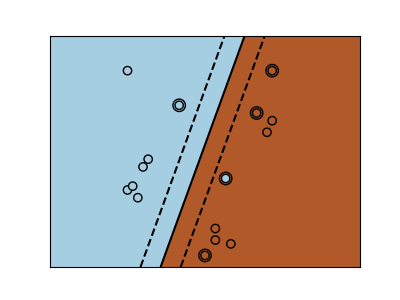
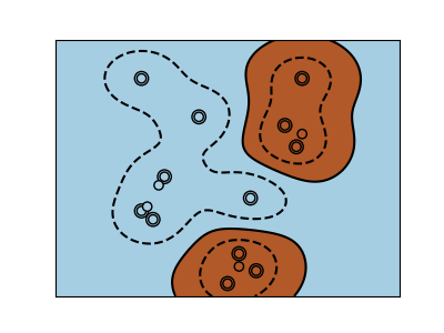
支持向量机：核函数¶

下面显示了三种不同类型的SVM核函数。当数据点不可线性分离时，多项式和RBF特别有用。 输入：

print(__doc__)


# 代码来源: Gaël Varoquaux
# 执照: BSD 3 clause

import numpy as np
import matplotlib.pyplot as plt
from sklearn import svm


# 我们的数据集与标签
X = np.c_[(.4, -.7),
          (-1.5, -1),
          (-1.4, -.9),
          (-1.3, -1.2),
          (-1.1, -.2),
          (-1.2, -.4),
          (-.5, 1.2),
          (-1.5, 2.1),
          (1, 1),
          # --
          (1.3, .8),
          (1.2, .5),
          (.2, -2),
          (.5, -2.4),
          (.2, -2.3),
          (0, -2.7),
          (1.3, 2.1)].T
Y = [0] * 8 + [1] * 8

# 图像的编号
fignum = 1

# 拟合模型
for kernel in ('linear', 'poly', 'rbf'):
    clf = svm.SVC(kernel=kernel, gamma=2)
    clf.fit(X, Y)

    # 绘制直线，点和最接近平面的向量
    plt.figure(fignum, figsize=(4, 3))
    plt.clf()

    plt.scatter(clf.support_vectors_[:, 0], clf.support_vectors_[:, 1], s=80,
                facecolors='none', zorder=10, edgecolors='k')
    plt.scatter(X[:, 0], X[:, 1], c=Y, zorder=10, cmap=plt.cm.Paired,
                edgecolors='k')

    plt.axis('tight')
    x_min = -3
    x_max = 3
    y_min = -3
    y_max = 3

    XX, YY = np.mgrid[x_min:x_max:200j, y_min:y_max:200j]
    Z = clf.decision_function(np.c_[XX.ravel(), YY.ravel()])

    # 将结果放入颜色图
    Z = Z.reshape(XX.shape)
    plt.figure(fignum, figsize=(4, 3))
    plt.pcolormesh(XX, YY, Z > 0, cmap=plt.cm.Paired)
    plt.contour(XX, YY, Z, colors=['k', 'k', 'k'], linestyles=['--', '-', '--'],
                levels=[-.5, 0, .5])

    plt.xlim(x_min, x_max)
    plt.ylim(y_min, y_max)

    plt.xticks(())
    plt.yticks(())
    fignum = fignum + 1
plt.show()

脚本的总运行时间：（0分钟0.229秒）